..
Swin transformers
Features
- Swin transformer can be used as a general purpose backbone for various computer vision tasks
- It produces an embedding for the image
- Earlier computer vision transformer architectures faced the problem of scalability as the computations are quadratic in nature
- Quadratic in relation to number of tokens (N)
- For images, this token size is high (based on # of patches)
Architecture
The model has the following blocks
- Patch partition
- Linear embedding
- Swin transformer block
- Contains windowed multi-self attention (W-MSA) and shifted window multi-self attentions (SW-MSA)
- Patch merging
Working example
Let’s consider a working example of one pass from each major block of the architecture. Consider input image of size: 32x32x3
Patch partition
- Divide the image into
patchesof4x4x3pixels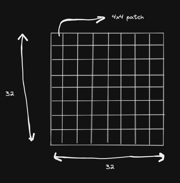
- In total we will have:
(32/4) * (32/4) = 64patches.
Linear embedding
- Flatten each patch to a vector. In this case the vector dimension for each patch would be
4*4*3 = 48. This vector is converted to an arbitrary dimension (called asCin the paper) using a vanilla neural network. For our example, let’s considerCas 64 - After this, you would have an image of size
(32/4) * (32/4) * 64- The overall image dimensions (height and width) will be reduced and each patch will be replaced with a feature vector of dimension
C. - The image size is now:
8 x 8 x 64
- The overall image dimensions (height and width) will be reduced and each patch will be replaced with a feature vector of dimension
Swin transformer block
- The image of above dimension is further divided into non-overlapping windows of
M x Mpatches. M is the number of windows. - For our example, let’s take M as 4
- Our window will contain
4 * 4 = 16patches, each with dimensionCas 64. 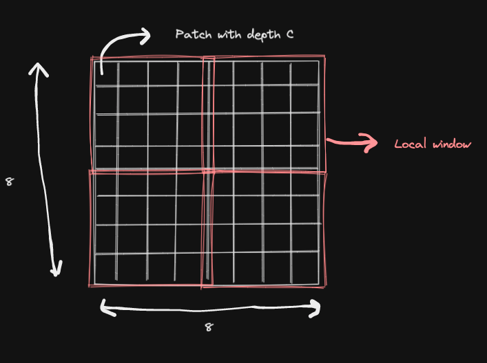
- Self attention is computed locally within each window. For our case, that would mean,
16 * 16 = 256dot products. Each patch attends to every other patch in the local window (i.e each patch attends to 16 other patches) - Query and Key matrix will have the dimensions:
16 * d.dis the query/key dimension.- Within a local window,
Querymatrix will only have16values
- Within a local window,
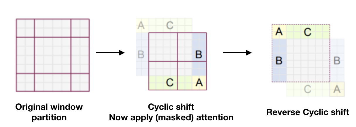
- This makes computation more scalable for large images and is called window based self attention
- Shift the windows to the bottom right by 2 patches. Compute self attention again.
Patch merging
- Merge patches in
2x2neighbourhood - This means, that we concatenate features of all the patches in
2x2neighbourhood. The resulting patch (or pixel) would now be of size4C, i.e256in our example. - A linear layer is applied to scale this back to
2C. i.e128for our example. - After patch merging, our image would now be of size
(8/2) * (8/2) * 2Ci.e4 x 4 x 128for our example.
For a real life model: swin_large_patch4_window7_224_22kto1k
- Patch size is 4
- Window size (M) is 7
- Input image size is
224 * 224 * 3